Using Machine Learning to Check if Breast Cancer Tumor is Malignant or Benign

The following article aims to use simple Machine Learning techniques to predict the classification of a breast cancer tumor and check if it’s Malignant or Benign. A step by step guide is given on how to carry out this task. The dataset can be found on UCI Machine Learning Repository. The features are computed from a digitized image of a fine needle aspirate (FNA) of a breast mass. The features describe characteristics of the cell nuclei present in the image. To understand the purpose of this model we need to understand the two classification possibilities present:

1. Malignant Tumor: A tumor that is cancerous
2. Benign Tumor: A tumor that is not cancerous

Our goal is to use the KNN algorithm to train a model using our dataset, and then based on that model devise predictions for whether a tumor will be malignant or benign based on it’s features.

Cleaning the Data

The dataset involves many variables and is not readily cleaned hence cleaning the dataset will involve more steps.

#import all the relevant libraries
import numpy as np
import pandas as pd
import matplotlib.pyplot as plt
import seaborn as sns
%matplotlib inline

#view the imported dataframe
df = pd.read_csv('data.csv')
df.head()

Dataset generated from the above code

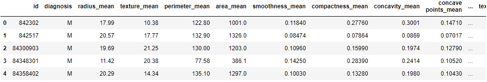
Now that the dataset has imported correctly we can notice that we have many metrics measuring different features. Due to the nature of the KNN algorithm it’s a good idea to scale the data in order to build a more accurate model.

#import scaling model and scale the data
from sklearn.preprocessing import StandardScaler
scaled = StandardScaler()
scaled.fit(df.drop(['id','diagnosis','Unnamed: 32'],axis=1))
df_scaled = scaled.transform(df.drop(['id','diagnosis','Unnamed: 32'],axis=1))

Training the Model

Now that our data is cleaned and scaled. It’s ready for training. We will achieve this by using scikit learn and hence need to import it’s relevant libraries.

#importing relevant libraries for the task
from sklearn.model_selection import train_test_split
from sklearn.neighbors import KNeighborsClassifier

#splitting data x are the categorical metrics and y is the prediction variable
X= df_scaled
y = df['diagnosis']

Our next job is to split the data into training and testing section. The training section will help the model to learn the pattern and the testing section will make it predict the nature of the tumor. We are using supervised learning once more and hence can verify our model using confusion and classification matrices.

X_train, X_test, y_train, y_test = train_test_split(X, y, test_size=0.3, random_state=42)

knn = KNeighborsClassifier(n_neighbors=1)
knn.fit(X_train,y_train)

Testing the Model

Now we will predict values using our model and then quantify them using a confusion matrix and classification matrix.

predictions = knn.predict(X_test)

from sklearn.metrics import confusion_matrix, classification_report,accuracy_score

print(classification_report(y_test,predictions))
print(confusion_matrix(y_test,predictions))
print(accuracy_score(y_test,predictions))

Accuracy measurements

Improving the Model

Our accuracy scores are really high but the KNN algorithm’s accuracy highly depends on the K value chosen for the metric. ( See KNN theory). Hence we will build a function that will help us identify a K value that gives the lowest error. Our function will find the various error intervals for each K value and we can visualize the function to find the results.

error_calc = []
for n in range(1,40):
    kn = KNeighborsClassifier(n_neighbors=n)
    kn.fit(X_train,y_train)
    predict = kn.predict(X_test)
    error_calc.append(np.mean(predict != y_test))

fig = plt.figure()
axes = fig.add_axes([1,1,1,1])
axes.plot(range(1,40),error_calc,marker='o',ls='--',markeredgecolor='red',lw=3)
axes.set_ylabel("% error")
axes.set_xlabel('Value of K')
axes.set_title("Error with different values of k")

Graph visualizing %error for various K values

From the graph we can deduce that the K value error is lowest for k=9 hence we will rebuild the model but with k=9 this time.

knn = KNeighborsClassifier(n_neighbors=9)
knn.fit(X_train,y_train)
predictions = knn.predict(X_test)

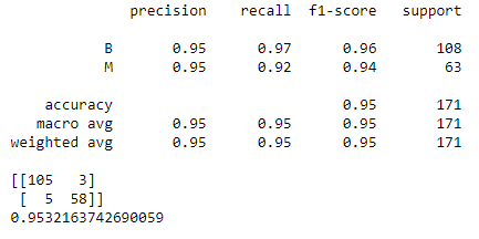
print(classification_report(y_test,predictions))
print(confusion_matrix(y_test,predictions))
conf_matrix = confusion_matrix(y_test,predictions)
print(accuracy_score(y_test,predictions))

Accuracy measurements

We can observe a really high accuracy for the model (97%) which proves that our model succeeded. We were also able to increase the accuracy of the model a bit more by choosing the best possible K value.